What You Have Built — and Where to Go Next

Recap the journey from hand-built loop to Gymnasium environment to neural-network policy, check your understanding, and explore the Farama ecosystem.

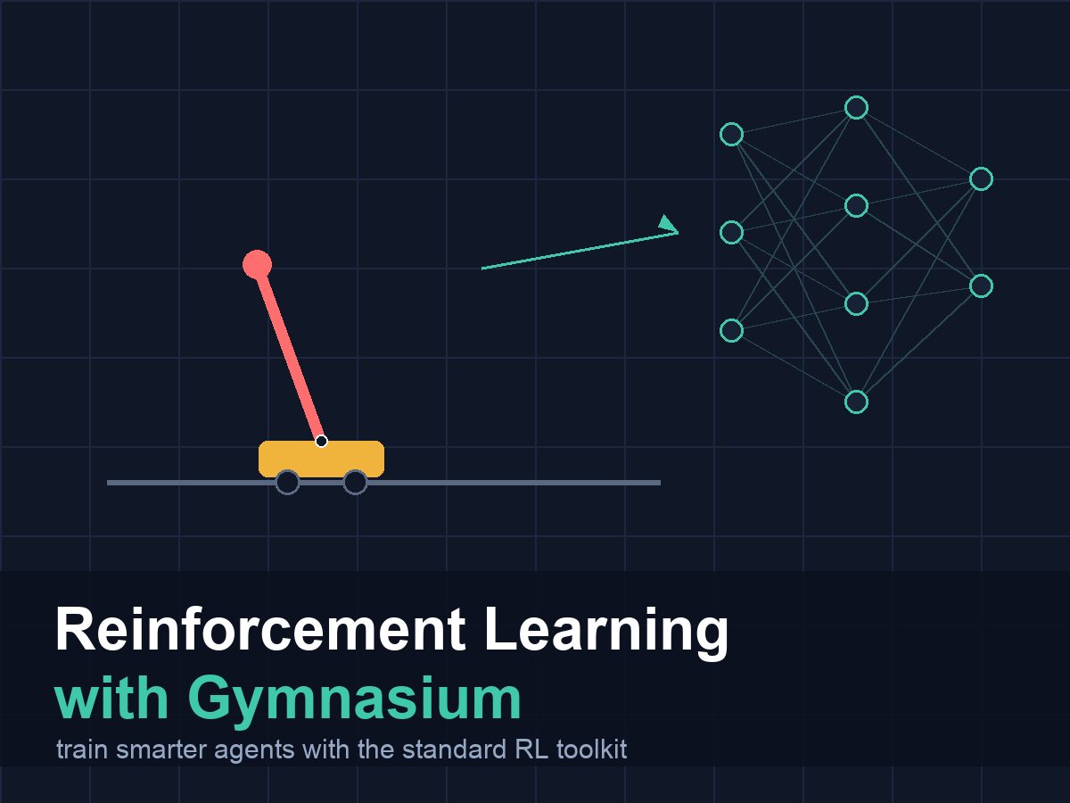
The Journey So Far

Let’s trace the full arc across both courses.

In the Reinforcement Learning for Beginners course, you started with a blank Python file and wrote everything yourself: the grid, the sensor, the reward function, the Q-table as a plain dictionary, the epsilon-greedy loop, and the Pico deployment code. That was deliberate — understanding every line is how the concepts stick.

In this course, you took those same ideas and moved them onto the tools the broader community uses. Here is what changed:

The environment interface:

• Before: state, reward, done = world.step(action) — a custom three-tuple, specific to your code
• After: obs, reward, terminated, truncated, info = env.step(action) — the Gymnasium standard, compatible with any Gymnasium-aware library

The agent:

• Before: a Python dictionary with 588 entries, updated by a hand-written Q-learning rule
• After: a neural network with thousands of parameters, trained by Stable-Baselines3’s PPO implementation

The deployment:

• Before: q_table.json loaded directly on the Pico
• After: nn_policy.json in the same format, produced by querying the neural network over all 588 states — so the same Pico loader still works

The physics did not change. The obstacles, the sensor, the rewards — all identical. What changed was the interface around them and the algorithm on top of them.

Concept Checklist

Work through this list. If anything feels uncertain, go back to the relevant lesson.

The Gymnasium API:

• I know that env.reset() returns (observation, info) and env.step(action) returns five values
• I can explain what terminated means and how it differs from truncated
• I know what observation_space and action_space are and how to inspect them
• I can use env.action_space.sample() to generate a random legal action

Custom environments:

• I can subclass gym.Env and implement reset() and step() correctly
• I know how to declare observation_space and action_space in __init__
• I can run check_env and interpret its output
• I know how to register an environment with gym.register and create it with gym.make

Wrappers and vectorisation:

• I know what RecordEpisodeStatistics adds to the info dict
• I can write a RewardWrapper that modifies rewards without editing the environment
• I understand that SyncVectorEnv batches observations and rewards across N environments

Stable-Baselines3:

• I can train a DQN or PPO agent with model.learn(total_timesteps=...)
• I understand that "MlpPolicy" means a fully-connected neural network
• I know how to save a model with model.save() and load it with Algorithm.load()
• I can evaluate a trained policy with evaluate_policy

Deployment:

• I understand why neural networks cannot run directly on a Pico
• I know the policy-table export trick: query the network over all states, save a JSON lookup table
• I understand the alternative for larger problems: run inference on a Raspberry Pi

What Happened to the Q-Table

The Q-table from the previous course was a dictionary with 588 keys and four float values per key. The neural network trained in this course is a function that takes a 4-dimensional input and produces four output values. Both are estimating the same thing: “how much future reward should I expect if I take action A from state S?”

The difference is that the neural network can generalise across similar states, and it can handle observations — camera images, raw sensor arrays, joint angles — that no table could hold. For the 588-state BurgerBot world, both approaches work. For a real robot navigating a building, only the neural network approach scales.

What’s Next

The Farama Ecosystem

You have learned Gymnasium, but Farama maintains a whole family of tools that extend it:

• PettingZoo — multi-agent environments with the same API style. If you want two BurgerBots navigating the same grid, PettingZoo is where to look.
• MuJoCo environments — physics-simulated robot control. HalfCheetah, Ant, and Humanoid are standard benchmarks for continuous-action RL.
• Minari — a dataset library for offline RL. Pre-recorded trajectories from expert policies, so you can train without interacting with the environment.
• Shimmy — compatibility wrappers for third-party environments like DeepMind Control Suite and ALE (Atari).

Robotics-Specific Next Steps

• ROS 2 and Gazebo — the professional robotics simulation stack. Your agent can control a simulated robot in a physics engine, then deploy to a real robot with the same code.
• MicroPython Robotics Projects — if you want to build more hardware to run policies on, this course covers motors, sensors, and chassis assembly.

Going Deeper on RL

• Proximal Policy Optimisation (PPO) — the algorithm you used in this course. The original paper is readable: “Proximal Policy Optimization Algorithms” by Schulman et al. (2017).
• Double DQN, Dueling DQN — the improvements on plain DQN mentioned in lesson 14 of the previous course. SB3’s DQN implements both by default.
• Soft Actor-Critic (SAC) — the algorithm of choice for continuous-action robotics. If your robot needs to control motor speed (a continuous value, not a discrete choice), SAC is where to look.
• CleanRL — single-file implementations of RL algorithms, excellent for reading and learning from. cleanrl.dev

Back to the Beginning

If you want to revisit where you started:

• Reinforcement Learning for Beginners — the foundation this course builds on. If anything in this course felt unclear, re-reading the tabular Q-learning implementation often helps.

One Last Thing

The move from a 100-line hand-written environment to a Gymnasium class is mostly renaming and restructuring. The concepts — states, actions, rewards, episodes, exploration, exploitation — do not change. The standard API just makes them portable.

The move from a Q-table to a neural network is more significant. The network is harder to inspect, harder to debug, and harder to guarantee correct behaviour from. But it scales to problems the table never could.

Knowing both is a genuine superpower. You can reach for a Q-table when the state space is small and interpretability matters. You can reach for SB3 and PPO when the problem is too large for a table. And you now know how to wrap any environment — grid-world, physical robot, simulated arm — in a standard interface that either approach can use.

Good luck building.

< Previous

You can use the arrows  ← → on your keyboard to navigate between lessons.