KevsRobots Learning Platform
Reinforcement Learning with Gymnasium
36% Percent Complete
Introduction
Why Gymnasium
The Gymnasium API in Depth
Building Your Own Environment
Scaling Up to Neural Networks
Q-Learning on Gymnasium
Port your tabular Q-learning agent from the previous course to run against CartPole-v1 — the same algorithm, now against a standard Gymnasium environment.
By Kevin McAleer, 7 Minutes
Page last updated June 14, 2026
The Bridge Lesson
This lesson is a bridge. You already know Q-learning — the update rule, epsilon-greedy exploration, and the Q-table dictionary. You already know Gymnasium — the five-return step(), the two-return reset(), and the space API.
Now let’s put them together. We will run your tabular Q-learning agent on CartPole-v1 using the Gymnasium API. No new concepts — just the familiar algorithm in the new standard wrapper.
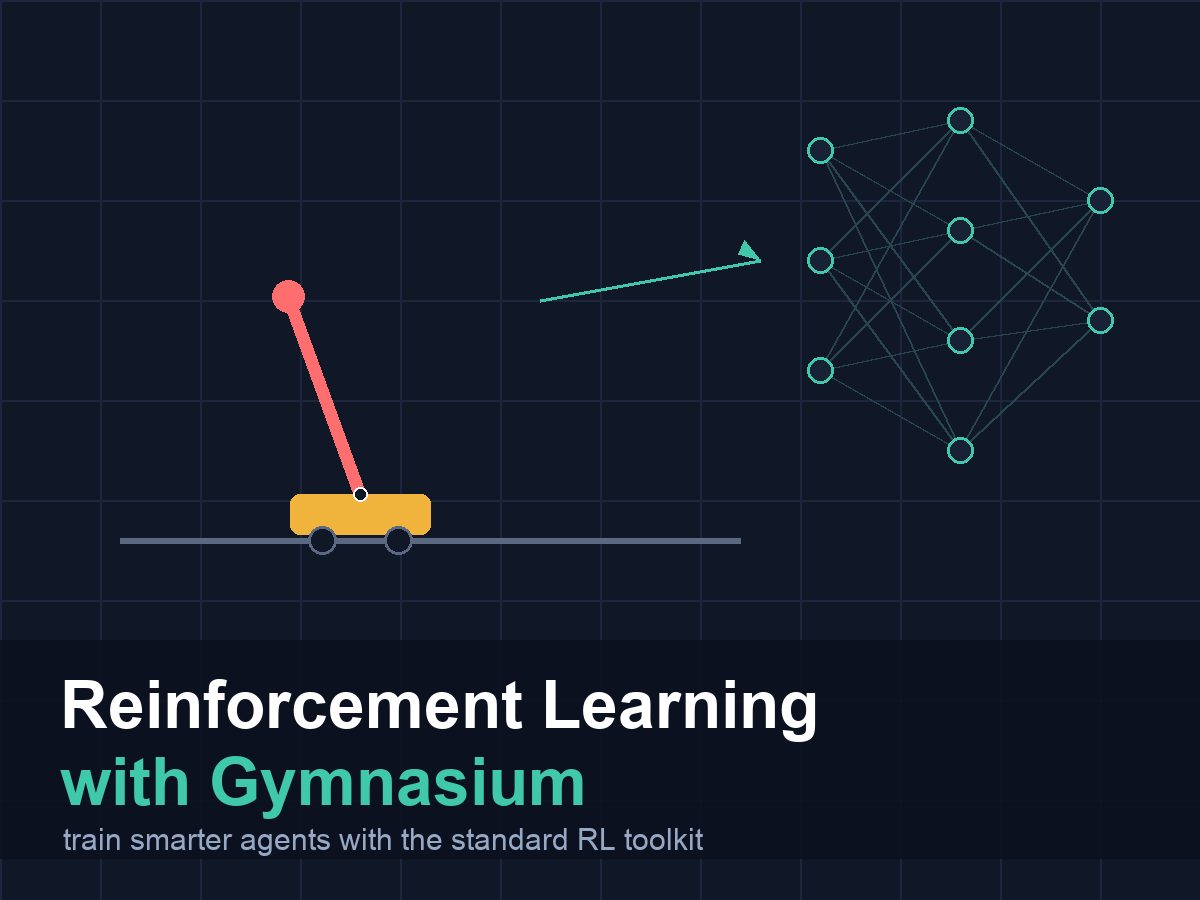
The interesting challenge: CartPole’s observation is a continuous Box(4) — four floating-point values. Your Q-table needs discrete keys. You need to bin those continuous values into discrete buckets.
You did exactly this in lesson 4 of the previous course with the discretize() function that converted ultrasonic sensor readings into “near”, “medium”, or “far”. Let’s do the same thing here.
Discretising CartPole’s Observation
CartPole gives you four continuous values per step:
- Cart position (roughly -4.8 to 4.8)
- Cart velocity (unbounded, practically -4 to 4)
- Pole angle (roughly -0.418 to 0.418 radians)
- Pole angular velocity (unbounded, practically -4 to 4)
We will bin each one into a small number of discrete buckets, then combine the four bucket indices into a tuple that becomes the Q-table key. This is the same idea as the previous course’s discretize() — just applied to four dimensions instead of one.
import numpy as np

# Number of bins per dimension. More bins = more states = slower learning.
# Fewer bins = coarser representation = faster learning but less precision.
N_BINS = 6

# Clip limits. Values beyond these get clamped to the edge bin.
# We use tighter limits than the space's true bounds because the agent
# rarely reaches the extreme ends before failing.
CLIP_LOW  = np.array([-2.4, -3.0, -0.25, -3.0])
CLIP_HIGH = np.array([ 2.4,  3.0,  0.25,  3.0])

def discretize(obs):
    """
    Convert a CartPole continuous observation into a tuple of bin indices.

    This is the same idea as the RL course's discretize() for ultrasonic
    readings, but applied to 4 dimensions at once using NumPy.
    """
    # Clip values to our expected range
    obs_clipped = np.clip(obs, CLIP_LOW, CLIP_HIGH)

    # Scale to [0, N_BINS - 1]
    # (obs - low) / (high - low) gives a value in [0, 1]
    # multiply by N_BINS and floor to get a bin index in [0, N_BINS - 1]
    scaled = (obs_clipped - CLIP_LOW) / (CLIP_HIGH - CLIP_LOW)
    bins = np.floor(scaled * N_BINS).astype(int)

    # Clamp to [0, N_BINS - 1] to handle any edge cases at the exact maximum
    bins = np.clip(bins, 0, N_BINS - 1)

    return tuple(bins)   # e.g. (3, 2, 4, 1)
A quick sanity check before using it:
import gymnasium as gym

env = gym.make("CartPole-v1")
obs, info = env.reset(seed=0)
print("Raw obs:", obs)
print("Discretized:", discretize(obs))
env.close()
# Raw obs: [ 0.04  -0.04   0.01  -0.02]
# Discretized: (3, 2, 3, 2)
The Complete Q-Learning Script
Here is the full training loop. You will recognise choose_action, update_q, and the episode loop from the previous course. The only changes are:
env.reset()returns(obs, info)not justobsenv.step()returns five values not three- Actions are integers (0 or 1) not strings
- States are tuples of bin indices not
(row, col, heading, sensor)tuples
import numpy as np
import gymnasium as gym
import random

# ── Discretisation settings ──────────────────────────────────────────────────
N_BINS  = 6
CLIP_LOW  = np.array([-2.4, -3.0, -0.25, -3.0])
CLIP_HIGH = np.array([ 2.4,  3.0,  0.25,  3.0])

def discretize(obs):
    obs_clipped = np.clip(obs, CLIP_LOW, CLIP_HIGH)
    scaled = (obs_clipped - CLIP_LOW) / (CLIP_HIGH - CLIP_LOW)
    bins = np.floor(scaled * N_BINS).astype(int)
    bins = np.clip(bins, 0, N_BINS - 1)
    return tuple(bins)

# ── Q-learning hyperparameters ───────────────────────────────────────────────
ALPHA         = 0.1     # learning rate
GAMMA         = 0.99    # discount factor
EPSILON_START = 1.0     # start fully random
EPSILON_MIN   = 0.01    # never go below 1 % random
DECAY_RATE    = 0.995   # per-episode decay (same as RL course)
NUM_EPISODES  = 500     # enough to see clear improvement

# ── Q-table ──────────────────────────────────────────────────────────────────
q_table = {}

def get_q(state):
    """Return Q-values for state, initialising to zero if unseen."""
    if state not in q_table:
        q_table[state] = [0.0, 0.0]   # one value per action (0=left, 1=right)
    return q_table[state]

def choose_action(state, epsilon):
    if random.random() < epsilon:
        return random.randint(0, 1)    # explore
    return int(np.argmax(get_q(state))) # exploit

def update_q(state, action, reward, next_state, terminated):
    current_q = get_q(state)[action]
    if terminated:
        # No future reward from a terminal state
        td_target = reward
    else:
        td_target = reward + GAMMA * max(get_q(next_state))
    get_q(state)[action] += ALPHA * (td_target - current_q)

# ── Training loop ─────────────────────────────────────────────────────────────
env = gym.make("CartPole-v1")
epsilon = EPSILON_START
recent_rewards = []

for episode in range(1, NUM_EPISODES + 1):
    obs, info = env.reset(seed=episode)
    state = discretize(obs)
    episode_reward = 0
    done = False

    while not done:
        action = choose_action(state, epsilon)
        next_obs, reward, terminated, truncated, info = env.step(action)
        next_state = discretize(next_obs)

        # Only pass terminated to update_q, not truncated.
        # A time-limit ending is not a true terminal state.
        update_q(state, action, reward, next_state, terminated)

        state = next_state
        episode_reward += reward
        done = terminated or truncated

    epsilon = max(EPSILON_MIN, epsilon * DECAY_RATE)
    recent_rewards.append(episode_reward)

    if episode % 50 == 0:
        avg = sum(recent_rewards[-50:]) / 50
        print(f"Episode {episode:4d}  avg(50)={avg:6.1f}  epsilon={epsilon:.3f}  states={len(q_table)}")

env.close()
print(f"\nFinal Q-table: {len(q_table)} states visited")
What to Expect
With 500 episodes and 6 bins, you should see something like:
Episode   50  avg(50)=  18.4  epsilon=0.778  states=142
Episode  100  avg(50)=  32.1  epsilon=0.606  states=287
Episode  150  avg(50)=  56.8  epsilon=0.472  states=391
Episode  200  avg(50)=  89.3  epsilon=0.368  states=430
Episode  300  avg(50)= 142.7  epsilon=0.223  states=461
Episode  400  avg(50)= 178.4  epsilon=0.135  states=472
Episode  500  avg(50)= 195.2  epsilon=0.082  states=478

Final Q-table: 478 states visited
CartPole gives a reward of +1 for every step the pole stays up. The maximum is 500 (the episode time limit). Reaching an average of 180+ by episode 500 with a tabular agent and only 6 bins per dimension is a good result.
Why This Matters
You just ran your tabular Q-learning algorithm on a completely different environment by:
- Writing a
discretize()function for the new observation type - Changing one string (
"CartPole-v1") and the action count from 4 to 2
The training loop itself did not change at all. That is the standard API working as designed.
Try It Yourself
- Increase
N_BINSfrom 6 to 10 and retrain. Does the agent reach a higher average reward? Does it take longer to converge? What happens tolen(q_table)? - Reduce
N_BINSto 3 and retrain. Is 3 bins enough information for the agent to learn a reasonable policy? - Add a
print(discretize(obs))at the start of each episode to watch the starting states. Are they all the same with a fixed seed? What happens if you remove the seed?
Common Issues
Problem: The average reward stays near 9-15 and never improves.
Solution: Your epsilon is decaying too fast. Try DECAY_RATE = 0.999 to explore for longer.
Why: With too few exploration steps the agent never visits enough states to build a useful Q-table.
Problem: The Q-table grows to tens of thousands of states.
Solution: Reduce N_BINS. More bins mean an exponential explosion in possible states. With 10 bins and 4 dimensions, that is up to 10,000 possible states — many of which the agent will never visit.
Why: The state space size with binning is N_BINS ** 4. With 6 bins that is 1,296 possible states; with 10 bins it is 10,000.
You can use the arrows ← → on your keyboard to navigate between lessons.
Comments