Meet Stable-Baselines3

Train DQN on CartPole in ten lines using Stable-Baselines3 — your first neural-network RL agent — and understand how MlpPolicy replaces the Q-table.

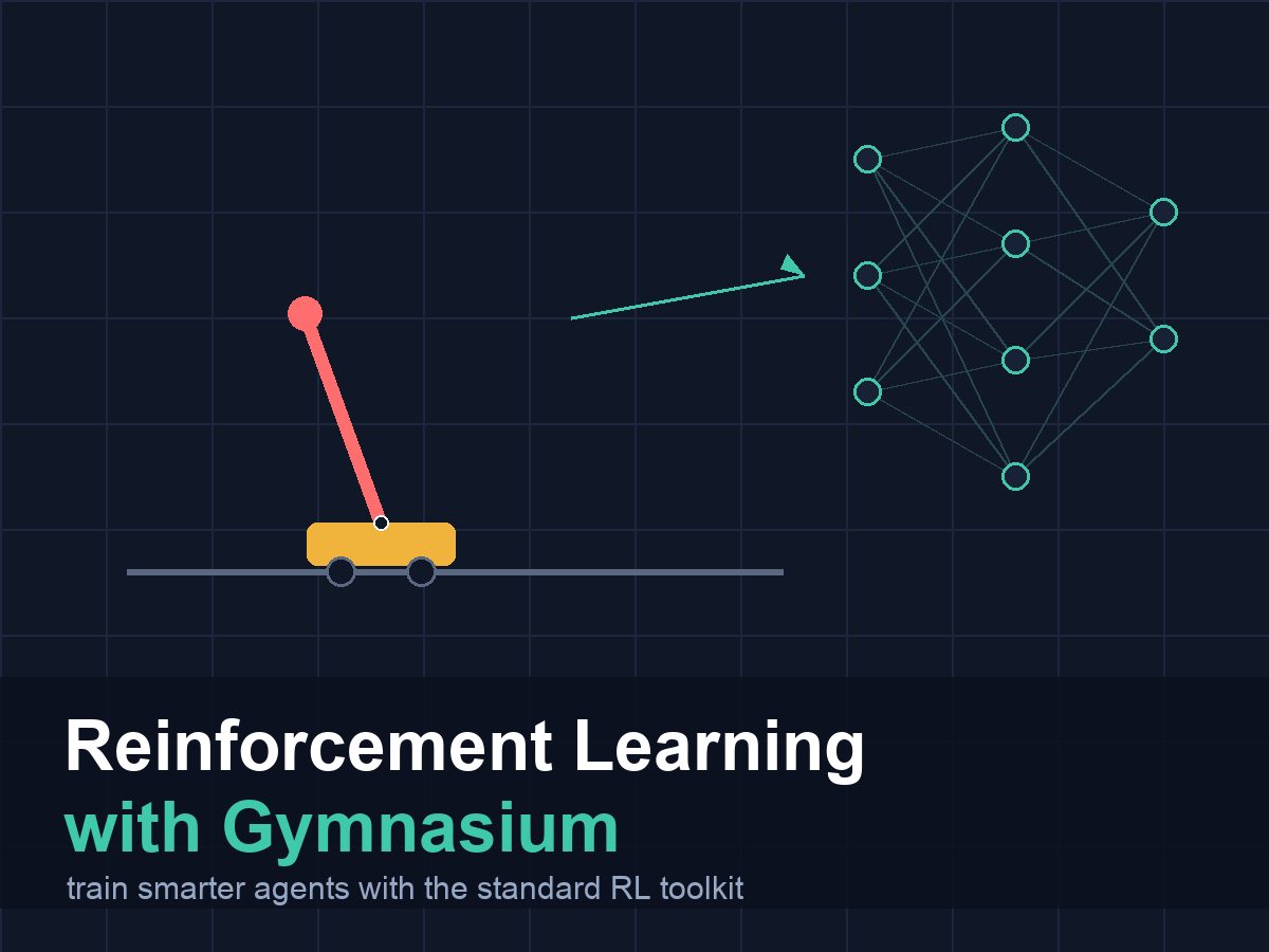
From Table to Network

In the previous course, lesson 14 ended with this question: “What happens when the state space is too large for a lookup table?”

The BurgerBot grid-world has 588 states. A lookup table with 588 entries is tiny. But even a low-resolution camera (say, 64x64 pixels in greyscale) has 256^4096 possible images — a number that dwarfs the number of atoms in the observable universe. No table can hold that.

The answer is to replace the table with a neural network. Instead of looking up Q[state][action], you compute network.forward(state) and get Q-values for all actions in one pass. The network generalises — if it has seen similar states during training, it can make a reasonable prediction on a new one.

Stable-Baselines3 (SB3) provides battle-tested implementations of the most widely-used deep RL algorithms. You do not need to write the network, the replay buffer, the loss function, or the optimizer. You hand SB3 an environment; SB3 trains an agent on it.

Installing Stable-Baselines3

If you installed it at the start of the course, it is already ready:

pip install stable-baselines3

Verify:

import stable_baselines3
print(stable_baselines3.__version__)   # 2.x.x

DQN on CartPole in Ten Lines

import gymnasium as gym
from stable_baselines3 import DQN

# Create the environment
env = gym.make("CartPole-v1")

# Create a DQN agent with a small multi-layer perceptron (MlpPolicy).
# SB3 inspects env.observation_space and env.action_space automatically.
model = DQN(
    "MlpPolicy",
    env,
    verbose=1,          # print training progress
    learning_rate=1e-3,
    buffer_size=10000,
)

# Train for 20,000 steps (takes about 20 seconds on CPU)
model.learn(total_timesteps=20000)

# Evaluate: run 5 episodes with the greedy policy
for episode in range(5):
    obs, info = env.reset()
    episode_reward = 0
    done = False
    while not done:
        action, _ = model.predict(obs, deterministic=True)
        obs, reward, terminated, truncated, info = env.step(action)
        episode_reward += reward
        done = terminated or truncated
    print(f"Episode {episode + 1}: reward = {episode_reward:.0f}")

env.close()

With 20,000 timesteps you should see episode rewards climbing from around 20 early in training to somewhere between 150 and 500 by the end. The network is learning.

What MlpPolicy Means

"MlpPolicy" tells SB3 to use a Multi-Layer Perceptron (MLP) — a standard fully-connected neural network — as the function approximator.

For DQN, the network takes the current observation as input and outputs one Q-value per possible action. The network learns to predict how much total future reward the agent will earn if it takes each action from the current state.

Compare this to the Q-table from the previous course:

# Tabular Q-learning (RL course, lesson 8):
# Look up the state in the table, get stored Q-values.
q_values = q_table[(row, col, heading, sensor)]   # exact lookup
action = argmax(q_values)

# DQN (what SB3 is doing internally):
# Feed the state to the network, get predicted Q-values.
q_values = network.forward(obs)   # neural network forward pass
action = argmax(q_values)

The interface is the same. The mechanism is different. And the scaling is dramatically better.

model.predict vs env.step

action, _states = model.predict(obs, deterministic=True)

model.predict takes a single observation (or a batch) and returns the best action according to the current policy. The second return value (_states) is only used for recurrent policies — you can ignore it for MLP policies.

deterministic=True means “use the greedy policy: always pick the highest Q-value action”. During training, SB3 handles exploration internally. During evaluation, you want the deterministic policy.

Key Hyperparameters

You do not need to tune these to get started, but it is good to know what they control:

model = DQN(
    "MlpPolicy",
    env,
    learning_rate=1e-3,      # how fast the network weights update
    buffer_size=50000,        # how many past transitions to store
    learning_starts=1000,     # how many random steps before training begins
    batch_size=32,            # transitions per gradient update
    gamma=0.99,               # discount factor — same gamma as the RL course
    exploration_fraction=0.1, # fraction of training spent reducing epsilon
    exploration_final_eps=0.05, # final epsilon (minimum exploration)
    target_update_interval=1000, # how often to sync the target network
    verbose=1,
)

The gamma and exploration_final_eps parameters are familiar from the previous course. SB3 handles all the mechanics around them.

Evaluating Cleanly with evaluate_policy

SB3 provides a utility function for rigorous evaluation:

from stable_baselines3.common.evaluation import evaluate_policy

mean_reward, std_reward = evaluate_policy(
    model,
    env,
    n_eval_episodes=10,
    deterministic=True,
)
print(f"Mean reward over 10 episodes: {mean_reward:.1f} +/- {std_reward:.1f}")

This runs exactly n_eval_episodes episodes and returns the mean and standard deviation of the episode rewards. Use this instead of a manual evaluation loop when you want a clean, comparable number.

Try It Yourself

1. Change total_timesteps=20000 to 5000 and retrain. How much does the final performance drop? This gives you a feel for how much training the agent needs.
2. Try from stable_baselines3 import PPO and replace DQN with PPO. Use n_steps=64 and n_envs=1. Does PPO reach the same performance? (PPO is an on-policy algorithm — it needs different hyperparameters.)
3. After training DQN, print model.policy. This shows the neural network architecture. How many layers does the default MLP have?

Common Issues

Problem: ValueError: You must use MultiInputPolicy when dealing with dictionary observation spaces Solution: Your environment uses a Dict observation space. Use "MultiInputPolicy" instead of "MlpPolicy". Why: SB3 has different policy classes for different observation types. MlpPolicy handles flat arrays (Box, Discrete, MultiDiscrete). MultiInputPolicy handles Dict spaces.

Problem: Training prints nothing even with verbose=1 Solution: SB3 only prints progress every log_interval timesteps. With very few timesteps (under 1000) you may not see output. Try verbose=2 for more frequent logging. Why: SB3’s progress reporting is tied to episode completions and log intervals, not raw step count.

Problem: UserWarning: Stable Baselines3 currently does not support Discrete observation spaces Solution: Wrap your Discrete observation in a Box: from gymnasium.wrappers import FlattenObservation. Or use MultiDiscrete (which SB3 does support). Why: DQN’s neural network expects a numeric array, not a single integer. SB3 handles MultiDiscrete by treating each component as a separate input feature.

< Previous Next >

You can use the arrows  ← → on your keyboard to navigate between lessons.